Tutorial 2: Velocity Boundary Conditions
Problem
This example solves for thermal convection with velocity boundary conditions imposed on the top surface within a given region of a sphere. This requires using the regional version of CitcomS.py.
Solution
You will use cookbook2.cfg. The parameters specify the number of time steps (61), the prefix of the output filenames (cookbook2), and how often outputs will be created (30):
 steps = 61
    monitoringFrequency = 30
    datafile = cookbook2
The solver.mesher facility has several properties involved in the generation of the computational mesh. Continue to use the default values for the physical portion of the domain in which you are interested. However, try modifying the layout of the mesh as shown:
 nprocx =  2
    nprocy =  2
    nodex  = 17
    nodey  = 17
    nodez  =  9
The solver.bc facility allows you to impose a uniform velocity across the top surface. You have a velocity which is purely in the colatitude direction with a non-dimensional velocity of 100 (see Equation 1.6 in the CitcomS User Manual for how to dimensionalize it):
 topvbc    =   1
    topvbxval = 100
In addition, the initial temperature field has a linear conductive profile. The amplitude of initial temperature perturbation is set to zero using the solver.ic facility
num_perturbations = 1
    perturbmag        = 0.0
Example: Velocity Boundary Conditions, cookbook2.cfg:
  [CitcomS]
    steps = 61                  ; number of time steps

    [CitcomS.controller]
    monitoringFrequency = 30    ; how often outputs are created

    [CitcomS.solver]
    datafile = cookbook2        ; prefix of output filenames

    # Modify the layout of the mesh.
    [CitcomS.solver.mesher]
    nprocx =  2
    nprocy =  2
    nodex  = 17
    nodey  = 17
    nodez  =  9

    # Impose a uniform velocity across the top surface.
    [CitcomS.solver.bc]
    topvbc    =   1
    topvbxval = 100

    # Modify the layout of the mesh.
    [CitcomS.solver.mesher]
    nprocx =  2
    nprocy =   2
    nodex  = 17
    nodey  = 17
    nodez  =  9

    # Impose a uniform velocity across the top surface.
    [CitcomS.solver.bc]
    topvbc    =   1
    topvbxval = 100
    topvbyval =   0

    # In addition, set the initial temperature perturbation to zero.
    [CitcomS.solver.ic]
    num_perturbations = 1
    perturbmag        = 0.0
Discussion
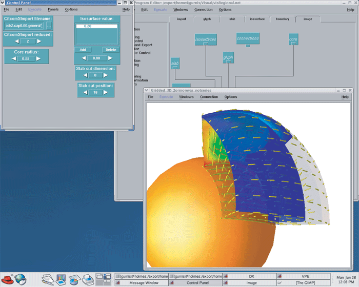
Using OpenDX to visualize the results (Figure 3 below), this model allows you to create a plate-driven convection in which there is a thermal upwelling on one wall, a thermal downwelling on another, and uniform horizontal velocity across the top. The downwelling is not exactly subduction because the default boundary conditions are close to zero shear stress on the boundaries. This means that there is a symmetrical downwelling in a vertical domain on the other side.
More tutorials are found in Chapter 6 of the CitcomS User Manual.


